Temporal Predictive Coding: A New Framework for Neural Processing of Dynamic Stimuli

Introduction

One of the most fascinating aspects of the brain is its ability to process and predict dynamic sensory inputs that continuously change over time. From tracking a moving object to predicting the next note in a melody, our brains are remarkably adept at temporal prediction. In a recent paper published in PLOS Computational Biology titled “Predictive coding networks for temporal prediction,” my colleagues and I proposed a new computational framework that may help explain how the brain accomplishes this feat.

Predictive coding has emerged as an influential theoretical model for understanding cortical function. The core idea is deceptively simple: the brain constantly generates predictions of incoming sensory inputs and compares these predictions with actual sensory data. Any mismatch results in prediction errors that drive learning and perceptual processing. This framework has successfully explained many neural phenomena and receptive field properties in visual cortex.

However, most previous predictive coding models have focused on static inputs, neglecting the temporal dimension that is crucial for real-world perception. Our work addresses this gap by extending predictive coding to the temporal domain while maintaining its elegant biological implementation.

The Temporal Predictive Coding Model

Generative Model and Free Energy

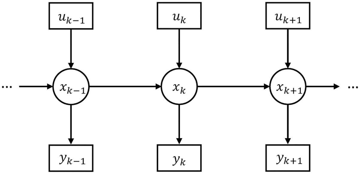
At the foundation of our temporal predictive coding (tPC) model is a Hidden Markov Model (HMM) structure, which assumes that observations are generated by hidden states that evolve according to a Markov process. Mathematically, we can express this generative model as:

$$x_k = A f(x_{k-1}) + B u_k + \omega_x$$

$$y_k = C f(x_k) + \omega_y$$

Where:

• $x_{k}$ is the hidden state at time $k$.
• $y_{k}$ is the observed sensory input at time $k$.
• $u_{k}$ is the control input at time $k$.
• $A$ is the dynamics matrix governing state transitions.
• $B$ is the control matrix.
• $C$ is the observation matrix.
• $f$ is a potentially nonlinear function.
• $\omega_x$ and $\omega_y$ are Gaussian process and observation noise.

The goal is to infer the current hidden state $x_{k}$ given the current observation $y_{k}$ and previous state estimate $y_{1:k-1}$. To achieve this, we formulate a variational free energy objective:

$$ \mathcal{F}k = \frac{1}{2}(y_k - C f(x_k))^T \Sigma_y^{-1} (y_k - C f(x_k)) + \frac{1}{2}(x_k - A f(\hat{x}{k-1}) - B u_k)^T \Sigma_x^{-1} (x_k - A f(\hat{x}_{k-1}) - B u_k) $$

This free energy can be understood as the sum of two weighted prediction errors:

1. Sensory prediction errors: The difference between observed and predicted sensory inputs $y_k - Cf(x_k)$.
2. Temporal prediction errors: The difference between the current state and the prediction from the previous state $x_k - Af(\hat{x}_{k-1}) - Bu_k$.

Each prediction error is weighted by the precision (inverse variance) of the corresponding noise distribution, ensuring that more reliable predictions carry more weight.

Neural Implementation

A crucial contribution of our work is showing how temporal predictive coding can be implemented in neural circuits using biologically plausible mechanisms. The neural dynamics for inferring the hidden state follow gradient descent on the free energy:

$$\tau \frac{d x_k}{d t} = -\epsilon_x + f'(x_k) \odot C^T \epsilon_y$$

Where $\epsilon_x$ and $\epsilon_y$ are precision-weighted prediction errors:

$$\epsilon_y = \Sigma_y^{-1} \left( y_k - C f(x_k) \right)$$

$$\epsilon_x = \Sigma_x^{-1} \left( x_k - A f(\hat{x}_{k-1}) - B u_k \right)$$

We proposed multiple neural circuit implementations of this model:

1. Network with explicit prediction error neurons: Where dedicated neurons represent prediction errors at each level of processing
2. Dendritic computing implementation: Where prediction errors are computed as differences between somatic and dendritic potentials
3. Single-iteration implementation: A simplified version that performs single updates per time step

Neural circuit implementation

Importantly, all of these implementations rely on local information and Hebbian plasticity. The synaptic weights are updated according to:

$$\Delta A = \eta \epsilon_x f(\hat{x}_{k-1})^T$$

$$\Delta B = \eta \epsilon_x u_k^T$$

$$\Delta C = \eta \epsilon_y f(x_k)^T$$

These update rules are Hebbian in nature because they depend only on the activities of pre- and post-synaptic neurons, making them biologically plausible.

Relationship to Kalman Filtering

An intriguing property of our model is its relationship to the Kalman filter, which is the optimal solution for linear Gaussian filtering problems. We demonstrated that both Kalman filtering and temporal predictive coding can be derived as special cases of Bayesian filtering, with the key difference being how they handle uncertainty.

The Kalman filter propagates uncertainty estimates through time, tracking the full posterior covariance at each step. In contrast, tPC approximates this by assuming a point estimate (Dirac distribution) for the previous state. Despite this simplification, our tPC model achieves comparable performance to the Kalman filter in tracking tasks while being computationally simpler and more biologically plausible.

For linear systems, the tPC dynamics at equilibrium yield:

$$ \hat{x}k^- = A\hat{x}{k-1} + Bu_k $$

$$\hat{x}_k = \hat{x}_k^- + K(y_k - C\hat{x}_k^-)$$

$$K = \Sigma_x C^T \left[C \Sigma_x C^T + \Sigma_y \right]^{-1}$$

This resembles the Kalman filter update equations but with a fixed gain matrix $K$ rather than a dynamically updated one based on posterior uncertainty.

Experimental Results

Performance in Linear Filtering Tasks

We tested our model on classic tracking problems, where the goal is to infer the hidden state (position, velocity, acceleration) of an object undergoing unknown acceleration based on noisy observations. Even with just a few inference steps between observations, tPC achieved performance approaching that of the optimal Kalman filter.

A key advantage of our model is its ability to learn the parameters of the generative model (matrices $A$, $B$, and $C$) using Hebbian plasticity. Even when starting with random matrices, tPC could learn to accurately predict observations. Interestingly, the model also implicitly encoded noise covariance information in its recurrent connections, without needing explicit representation of precision matrices.

Motion-Sensitive Receptive Fields

Perhaps most excitingly, when trained on natural movies, our tPC model developed spatiotemporal receptive fields resembling those observed in the visual cortex. These fields exhibited Gabor-like patterns and direction selectivity, a hallmark of motion-sensitive neurons in early visual areas.

Nonlinear Extensions

We extended the model to handle nonlinear dynamics by incorporating nonlinear activation functions. When tested on a simulated pendulum task, the nonlinear tPC significantly outperformed the linear model, accurately predicting the pendulum’s motion even at extreme angles where nonlinear effects are strongest.

Implications and Future Directions

Our temporal predictive coding framework has several important implications:

1. It provides a biologically plausible explanation for how the brain processes dynamic stimuli and performs temporal predictions.
2. It demonstrates that complex temporal filtering operations can be implemented in neural circuits using simple, local computations.
3. It offers a unified framework that connects normative theories of perception (Bayesian inference) with mechanistic models of neural circuits.
4. It suggests that the same computational principles might underlie both static and dynamic sensory processing in the brain.

Conclusion

The temporal predictive coding model we’ve developed bridges an important gap in our understanding of how the brain processes dynamic sensory inputs. By extending predictive coding to the temporal domain while maintaining its biological plausibility, our model provides a compelling computational mechanism for temporal prediction in neural circuits.

The fact that our model develops receptive fields resembling those in the visual cortex and approximates optimal filtering solutions suggests that temporal predictive coding may indeed capture fundamental principles of neural computation in the brain. As we continue to refine these models and test them against empirical data, we hope to gain deeper insights into the remarkable predictive capabilities of the brain.

This blog is based on the paper “Predictive coding networks for temporal prediction” by Beren Millidge, Mufeng Tang, Mahyar Osanlouy, Nicol S. Harper, and Rafal Bogacz, published in PLOS Computational Biology, April 2024. Link to the paper